Chapter 12 Repeated Measures and Longitudinal Data

This week, our goals are to…

1. Identify and characterize longitudinal data structures.

2. Apply already-learned concepts about nested/grouped data to the analysis of longitudinal data.

3. Analyze longitudinal and repeated measures data using fixed and random effects.

Announcements and reminders

1. Please email Nicole and Anshul to schedule your Oral Exam #3. The course calendar shows the ideal dates to do Oral Exam #3.

12.1 Longitudinal data structures

In the last few chapters, we learned about how to use fixed and random effects models to model cross-sectional data on observations that are clustered into groups. For example, we looked at data on students whose MCAT scores were each measured one time, and these students were grouped into three classrooms. We had to account for this grouping because the data we had from each observation (student) was dependent on that observation’s group (classroom). That is why we could not use OLS (ordinary least squares) linear regression for this data without correcting for grouping.

We also learned about how to add level 1 and level 2 independent variables into the model. Level 1 variables are those at the individual level such as hours spent studying. Level 2 variables are those at the group level such as teacher quality.

In this chapter, we will use these same tools to answer a repeated measures research question, in which we have multiple measurements of the dependent variable for each observation. As you will see as you read the chapter, this creates a data structure that is very similar to the clustered/nested data we looked at before. However, the data generating mechanism in this case is different.

In this chapter, after exploring the similarities and differences between cross-sectional and longitudinal data, we will use fixed effects and random effects regression models (the same regression models we learned over the last few chapters) to fit longitudinal data.

We will begin by comparing what longitudinal, cross-sectional, and nested data looks like. Then, we will look at some example data that has repeated measures and consider how this is analogous to cross-sectional nested data.

12.1.1 Longitudinal compared to cross-sectional data

It is important for us to understand the distinction between longitudinal and cross-sectional data. If you wish, you can read the following short articles which describe the two types of data and research designs (not required):

• Longitudinal vs cross-sectional studies, Learning Hub – This contains a useful table that compares the two types of data and research designs.
• Cross-sectional vs. longitudinal studies, Institute for Work & Health – This contains a useful example of the two types of data and research designs.

As you can see from the resources above, not only is the organization of the data different between cross-sectional and longitudinal, but the data generating mechanism/process is also different. In cross-sectional studies, we examine our outcome of interest only once in each observation (which is an individual person in many cases), but in longitudinal studies we examine our outcome of interest multiple times in each population. These differences in study design generate different structures of data.

So far in this chapter, we have used the terms repeated measures and longitudinal to refer to similar types of studies and data. We can think of repeated measures as one type of longitudinal data. It is fine to think of these as being extremely similar to one another.

12.1.2 Review of nested data

Before we continue our exploration of longitudinal research designs and data structures, let’s review some of the basic framework of nested or multilevel data that we learned before.

In the practice data we used before, students were nested within classrooms, so there were two levels of data:

Level 1	Level 2
Students	Classrooms

Nested data is also referred to as multilevel data and regression techniques to model this data are referred to collectively as multilevel modeling.

We learned that we can also have more than two levels of data. If we had data on students that are within classrooms that are in turn within schools. Then we would have three nested levels of data:

Level 1	Level 2	Level 3
Students	Classrooms	Schools

Each of these levels of data can have its own set of independent variables.

Previously, we referred to Level 1 as the individual level and Level 2 as the group level. That is because students were “grouped” into classrooms. The example dataset on students’ MCAT scores and hours spent studying contains cross-sectional data, since each student was measured only once and at approximately the same point in time.

12.1.3 Example research design – sleep study

Throughout this chapter, we will use a single dataset for all of our examples. This dataset is called sleepstudy and it is part of the lme4 package. The example presented in this chapter is adapted from Bates et al.²⁰³

You can run the code below to open up the data and follow along as you read this chapter:

if (!require(lme4)) install.packages('lme4')
library(lme4)

data(sleepstudy)

Once you run the code above, you will see that the sleepstudy data has been added to your Environment in RStudio.

Here is some information about the sleepstudy data, from the literature on the lme4 package:²⁰⁴

…we will work with a data set on the average reaction time per day for subjects in a sleep deprivation study (Belenky et al. 2003). On day 0 the subjects had their normal amount of sleep. Starting that night they were restricted to 3 hours of sleep per night. The response variable, Reaction, represents average reaction times in milliseconds (ms) on a series of tests given each Day to each Subject…

You can also run the command ?sleepstudy in R on your own computer to see more information about the dataset.

The research question we are trying to answer with this data is:

What is the relationship between reaction time and days of sleep deprivation?

As a first step, please visually inspect this data on your own (in RStudio on your own computer) by running the following code:

View(sleepstudy)

Below, the first 20 rows of the dataset are displayed:

head(sleepstudy,n=20)

##    Reaction Days Subject
## 1  249.5600    0     308
## 2  258.7047    1     308
## 3  250.8006    2     308
## 4  321.4398    3     308
## 5  356.8519    4     308
## 6  414.6901    5     308
## 7  382.2038    6     308
## 8  290.1486    7     308
## 9  430.5853    8     308
## 10 466.3535    9     308
## 11 222.7339    0     309
## 12 205.2658    1     309
## 13 202.9778    2     309
## 14 204.7070    3     309
## 15 207.7161    4     309
## 16 215.9618    5     309
## 17 213.6303    6     309
## 18 217.7272    7     309
## 19 224.2957    8     309
## 20 237.3142    9     309

Before we look individually at each variable (column), let’s take an overall look at how the data is structured and the mechanism that generated it. The reaction time of each subject (participant in the study) was measured ten times, on ten separate days. Each of these measurements appears in its own separate row in the data. Therefore, there are ten rows for each subject in the data.

Now we can look at the variables. Let’s start with Subject on the right side. The identity of the first subject in the data is 308. That is the subject identification number. The name of the subject could have been here instead of a number, and nothing would be different about the data or the study. You can see that there are ten observations (rows of data) for Subject 308, ten rows for Subject 309, and so on for all subjects in the data.

The Reaction variable contains the repeated measure for each subject that was taken ten times. This is what makes the data longitudinal, because each subject was observed (measured) multiple times. In this case, the Reaction variable is measuring the reaction time of the subject on a particular day.

Finally, the Days variable tells us which day each measurement occurred.

Here are some examples, picked out from the data:

• In row 6 of the data, we see that when Subject 308 had been sleep deprived for 5 days, their reaction time was 414.6901 milliseconds.
• In row 11, we see that when Subject 309 had been sleep deprived for 0 days (meaning at the very start of the study), their reaction time was 222.7339 seconds.

Let’s review the key details:

• Reaction is the dependent variable of interest. It is a repeated measure of reaction time over the course of ten days for each subject in the study.
• Days is the independent variable of interest. It records the number of days since the start of the study and tells the day on which the Reaction measurement was taken on each subject. Days tells us the number of nights for which the participant has been sleep deprived.
• Subject identifies each participant in the study and is the group variable in the language of multilevel modeling (more on this is below).

12.1.4 Individuals as groups

Keeping in mind the research design you just read about, as well as the review material on nested data structures, let’s consider how the longitudinal data generating process described above actually led us to create nested data.

The researchers wanted to study how reaction time varied with increasing days of sleep deprivation. So, of course, they had to measure each person multiple times. They decided that they would measure Reaction once every 24 hours, and before each measurement they would sleep-deprive their subjects even more than before. They of course kept track of how many days each subject was studied for when they made each measurement, and that’s what created the Days variable.

It turns out that this research design created nested data that is very similar to the nested data we have seen before in this textbook. In this case, reaction times and days are nested within individual subjects. Since we have ten repeated measures of Reaction, each subject appears in the data ten times. It is important for each measurement to be on its own row, as it is right now.²⁰⁵

In our MCAT scores example from before—which used cross-sectional data—students were nested within classrooms. In longitudinal data, measurements of subjects are nested within those very same subjects. The tables below might help make these analogous situations clearer.

Levels of data:

Study Type	Level 1	Level 2
Cross-sectional	Subjects (students)	Groups (classrooms)
Longitudinal	Measurements (reaction time)	Subjects (study participants)

As you can see, in the language of multilevel modeling, we still have two levels of data. But the way that the we generated these two levels means that one study is cross-sectional and the other is longitudinal.

Also like before, we have independent variables at each level of data within our nested hierarchy. In the table below, you’ll see the same independent variables for the MCAT cross-sectional data we used before as well as the analogous variables for the new sleepstudy longitudinal data.

Variables at each level:

Data Type	Dependent Variable	Level 1 Independent Variables	Level 2 Independent Variables
Cross-Sectional	MCAT score percentile	Hours spent studying	Teacher quality
Longitudinal	Reaction time	Days of sleep deprivation	Age and sex of participant

Note that age and sex of participant are not included in the sleepstudy data, but those are examples of characteristics of each Subject that would be Level 2 variables, if we had that information.

Let’s review the cross-sectional the longitudinal research questions that we can ask with these two types of data:

• Cross-sectional: What is the relationship between MCAT score and hours spent studying; controlling for classroom and teacher quality?
• Longitudinal / repeated measure: What is the relationship between reaction time and days of sleep deprivation; controlling for subject, subject’s age, and subject’s sex?

To answer the question to the cross-sectional research question above, we needed to know the regression coefficient estimate (slope) of the hours spent studying variable. This told us the relationship between hours spent studying and MCAT score.

Analogously, to answer the longitudinal research question above, we need to learn the regression coefficient estimate of the days of sleep deprivation variable. This will tell us the relationship between days of sleep deprivation and reaction time.

The computer doesn’t “know” whether we are doing a cross-sectional or repeated measures research design. All it “knows”—once we tell it—is that this is multilevel nested data.

12.1.5 Visualization

Using some visualizations can help us further understand the analogous nature of nested cross-sectional data and repeated measures longitudinal data.

Let’s begin by yet again visualizing the MCAT score data that we have been using as an example of a multilevel cross-sectional study. This time, we will make a separate scatterplot for each of the three classrooms in our data (it is not required for you to understand the code used to do this):

study <- c(50,53,55,53,57,60,63,65,63,67,70,73,75,73,77)
mcat <- c(77,76,77,78,79,73,74,73,75,75,63,64,65,66,70)
classroom <- c("A","A","A","A","A","B","B","B","B","B","C","C","C","C","C")
prep <- data.frame(study, mcat, classroom)

if (!require(ggplot2)) install.packages('ggplot2')
library(ggplot2)
ggplot(prep, aes(x = study, y = mcat)) + geom_point(color = "blue", alpha = 0.7) + geom_smooth(method = "lm", color = "black") + theme_bw() + facet_wrap(~classroom)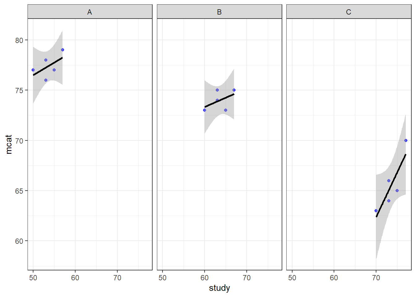

Above, we see the plotted relationship between mcat and study. By adding + facet_wrap(~classroom) to the code, we get a separate scatterplot for each classroom. This shows the very same trends in each classroom that we have examined in previous chapters. As hours of study increases, MCAT score also increases. The dependent variable mcat is on the vertical axis, the independent variable hours is on the horizontal axis, and there is a separate plot made for each level of the group variable classroom. Each plotted point (blue dot) is a student, which is the unit of observation at Level 1.

Since there were only three classrooms, it was easy to just look at all data in a single large scatterplot. However, if we have more than just a few groups, looking at all of them on a single scatterplot might not be very helpful. For the sleepstudy data, we could make a single scatterplot with a separate line for each subject, but it would be hard to read.

Let’s make a similar visualization for the sleepstudy data, in which we have separate scatterplots for each participant. Here’s the code to do that (which you are not required to understand):

if (!require(ggplot2)) install.packages('ggplot2')
library(ggplot2)

ggplot(sleepstudy, aes(x = Days, y = Reaction)) + geom_point(color = "blue", alpha = 0.7) + geom_smooth(method = "lm", color = "black") + theme_bw() + facet_wrap(~Subject)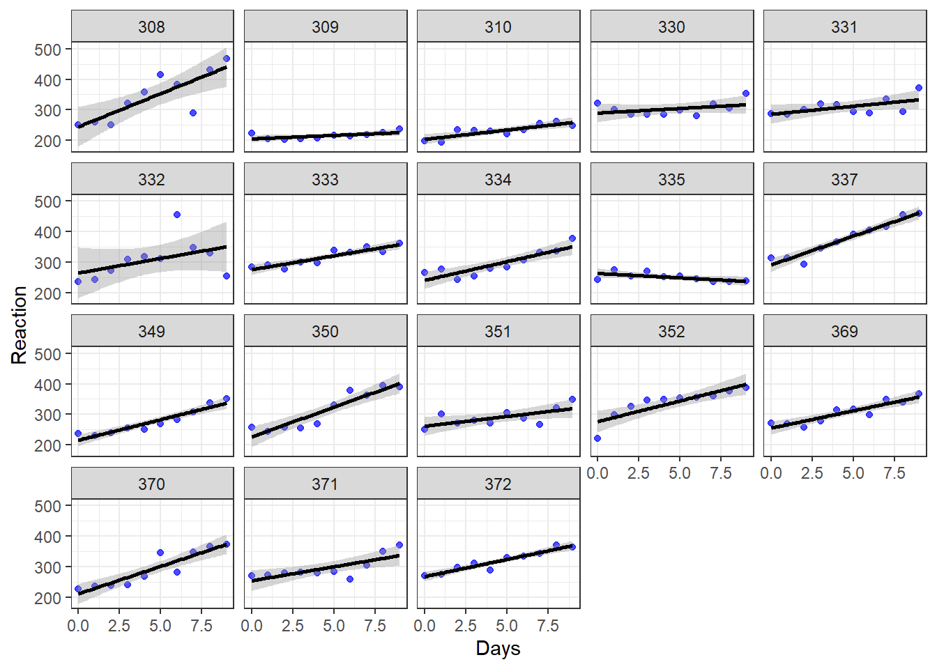

Above, we see the plotted trend between Reaction and Days separately for each of the 18 subjects in the study. We see that for most—but not all—of the subjects, as days of sleep deprivation increases, reaction time also increases. The dependent variable Reaction is on the vertical axis, the independent variable Days is on the horizontal axis, and there is a separate plot made for each level of the group variable Subject. Each plotted point (blue dot) is a measurement of reaction time.

Remember:

• In the cross sectional data, each plotted point is an individual subject.
• In the longitudinal data, each plotted point is a single measurement, and there are many measurements taken on each individual subject.

Note that if we wanted to create plots for only a subset of our dataset (which could be useful if the dataset is really big), we could run the following code (the result is not shown but you can run it in R on your own computer to see):

ggplot(sleepstudy[1:50,], aes(x = Days, y = Reaction)) + geom_point(color = "blue", alpha = 0.7) + geom_smooth(method = "lm", color = "black") + theme_bw() + facet_wrap(~Subject)

Above, the dataset we used is sleepstudy[1:50,] instead of just sleepstudy like we used earlier. This selects just the first 50 rows from the dataset sleepstudy and treats it as a new dataset. You will need to use this trick in this chapter’s assignment!

Let’s compare the types of data in these two analogous visualizations above and their corresponding research scenarios:

	Cross-Sectional	Longitudinal
Vertical Axis	mcat	Reaction
Horizontal Axis	hours	Days
Outcome of Interest	mcat	Reaction
Key Independent Variable	hours	Days
Level 1 unit of observation	student	measurement of reaction
Level 2 unit of observation	classroom	Subject
Group Variable	classroom	Subject

In both scenarios above, the outcome of interest is always on the vertical axis and the key independent variable of interest is on the horizontal axis. But the group (level 2) variable is very different and that’s what makes one cross-sectional and the other longitudinal.

In the plots above, we looked within each subject in our data to look at trends. We can also try to look across subjects for an overall trend using a boxplot:

boxplot(Reaction ~ Days, data = sleepstudy)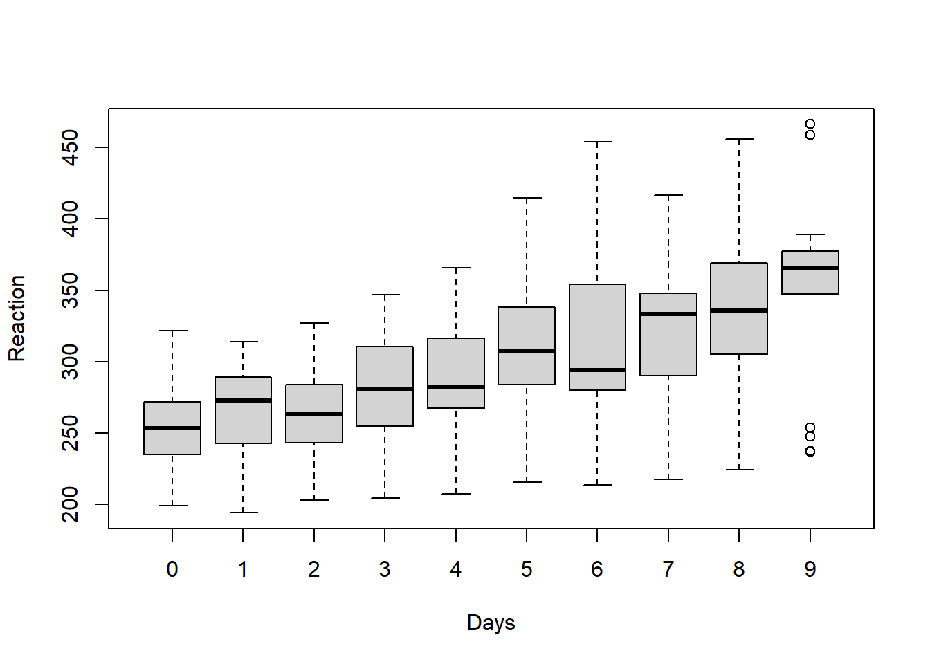

Above, we see that overall average reaction times appear to go up as the number of days increases. Of course, it important to remember that all of these plots are just exploratory and do not account for any confounding variables or other sources of bias in the analysis.

12.2 Intra-class correlation

Just like with cross-sectional multilevel data, the repeated measures made on each subject in longitudinal data are very likely to be correlated with each other. Let’s review this concept below:

• In our MCAT scores example data, MCAT scores of students (level 1) were more likely to be similar to each other if they came from the same classroom (level 2).

• Likewise, in the sleepstudy data, reaction times (level 1) were more likely to be similar to each other if they came from the same subject (level 2).

We can again use the intra-class correlation (ICC) to calculate how similar reaction times are to each other when taken from the same subject. The key concepts related to ICC that we learned before still apply.

Like before, to calculate ICC, we will make a null model that only allows us to look at variance the Level 1, Level 2, and total variance in our data. Remember that the null model is one in which we only have the dependent variable and the grouping variable. There are no independent variables included in the model.

Here is the code to make the null model for the sleepstudy research question we want to answer:

summary(null <- lmer(Reaction ~ 1 + (1|Subject), data = sleepstudy))

## Linear mixed model fit by REML ['lmerMod']
## Formula: Reaction ~ 1 + (1 | Subject)
##    Data: sleepstudy
## 
## REML criterion at convergence: 1904.3
## 
## Scaled residuals: 
##     Min      1Q  Median      3Q     Max 
## -2.4983 -0.5501 -0.1476  0.5123  3.3446 
## 
## Random effects:
##  Groups   Name        Variance Std.Dev.
##  Subject  (Intercept) 1278     35.75   
##  Residual             1959     44.26   
## Number of obs: 180, groups:  Subject, 18
## 
## Fixed effects:
##             Estimate Std. Error t value
## (Intercept)   298.51       9.05   32.98

As you can see above, Reaction is our dependent variable and Subject is our grouping variable. We have left out any independent variables for now. We have put a 1 in the formula in two places to indicate that we want separate “random” intercepts for each Subject. The computer figured out that we have 18 subjects, which are our groups (level 2). And it figured out that we have 180 total reaction measurements (level 1).

Let’s review how we calculated ICC before:

\[\rho=\frac{\text{Variance at highest level}}{\text{Total variance}}=\frac{\text{Group variance}}{\text{Group variance}+\text{Residual Variance}}\]

Keeping in mind that in our longitudinal study, a “group” is now a subject, let’s rewrite this equation:

\[\rho=\frac{\text{Variance at highest level}}{\text{Total variance}}=\frac{\text{Subject variance}}{\text{Subject variance}+\text{Residual Variance}}\]

In our null model above:

• Subject variance = 1278
• Residual variance = 1959

\[\rho=\frac{1278}{1278+1959} = 0.395\]

This value tells us how correlated the reaction measurements from any one subject are with each other. This tells us how non-independent our data are. Such a high ICC means that we do need to use a regression model that accounts for clustering/nesting such as fixed effects or random effects. We cannot use OLS linear regression, because our data violate the independence assumption required to use OLS regression. Furthermore, using OLS regression would make us susceptible to Simpson’s Paradox, meaning that we might accidentally find a false trend in our data by failing to look at each group separately.

Like before, we can have R double-check our ICC calculation for us:

if (!require(performance)) install.packages('performance')
library(performance)
performance::icc(null)

## # Intraclass Correlation Coefficient
## 
##     Adjusted ICC: 0.395
##   Unadjusted ICC: 0.395

It is important to always do an ICC calculation at the start of any analysis you do that has grouped data. In the case of longitudinal data, which is this chapter’s focus, I recommend that in your regression model, you should always account for measurements that are grouped by subject, even if the ICC is low.

12.3 Fixed effects for repeated measures

Now that we have understood how our data was generated and how it is structured, we can finally turn to the issue of modeling our data and answering our research question. We will begin by using a fixed effects regression model. Remember: fixed effects just means adding a dummy variable for each group.

In this section, we will follow the very same procedure that we followed when fitting a fixed effects model to our MCAT scores example data. First, we will use the lm() command to fit an OLS linear regression model with fixed effects for each subject. Then, we will use the plm() command to fit the same model.

12.3.1 lm() fixed effects

The first regression model will make in most situations is an OLS linear regression model. So we’ll again start there.

We will run this with the following familiar code:

reg1 <- lm(Reaction ~ Days + Subject, data = sleepstudy)
summary(reg1)

## 
## Call:
## lm(formula = Reaction ~ Days + Subject, data = sleepstudy)
## 
## Residuals:
##      Min       1Q   Median       3Q      Max 
## -100.540  -16.389   -0.341   15.215  131.159 
## 
## Coefficients:
##              Estimate Std. Error t value Pr(>|t|)    
## (Intercept)  295.0310    10.4471  28.240  < 2e-16 ***
## Days          10.4673     0.8042  13.015  < 2e-16 ***
## Subject309  -126.9008    13.8597  -9.156 2.35e-16 ***
## Subject310  -111.1326    13.8597  -8.018 2.07e-13 ***
## Subject330   -38.9124    13.8597  -2.808 0.005609 ** 
## Subject331   -32.6978    13.8597  -2.359 0.019514 *  
## Subject332   -34.8318    13.8597  -2.513 0.012949 *  
## Subject333   -25.9755    13.8597  -1.874 0.062718 .  
## Subject334   -46.8318    13.8597  -3.379 0.000913 ***
## Subject335   -92.0638    13.8597  -6.643 4.51e-10 ***
## Subject337    33.5872    13.8597   2.423 0.016486 *  
## Subject349   -66.2994    13.8597  -4.784 3.87e-06 ***
## Subject350   -28.5312    13.8597  -2.059 0.041147 *  
## Subject351   -52.0361    13.8597  -3.754 0.000242 ***
## Subject352    -4.7123    13.8597  -0.340 0.734300    
## Subject369   -36.0992    13.8597  -2.605 0.010059 *  
## Subject370   -50.4321    13.8597  -3.639 0.000369 ***
## Subject371   -47.1498    13.8597  -3.402 0.000844 ***
## Subject372   -24.2477    13.8597  -1.750 0.082108 .  
## ---
## Signif. codes:  0 '***' 0.001 '**' 0.01 '*' 0.05 '.' 0.1 ' ' 1
## 
## Residual standard error: 30.99 on 161 degrees of freedom
## Multiple R-squared:  0.7277, Adjusted R-squared:  0.6973 
## F-statistic: 23.91 on 18 and 161 DF,  p-value: < 2.2e-16

Above, Reaction is our dependent variable. Days and Subject are our independent variables. Note that Subject is coded as a categorical variable.²⁰⁶ Therefore, a separate dummy variable is added to our model for each subject in the data. This creates a separate intercept for each subject. This is equivalent to the varying intercepts model that we made previously with the MCAT score data.

Note that if we had additional variables like sex and age of each subject, we could include those in the model like this:

reg1 <- lm(Reaction ~ Days + Subject + sex + age, data = sleepstudy)

We can also see the results with 95% confidence intervals included:

if (!require(jtools)) install.packages('jtools')
library(jtools)

summ(reg1, confint = TRUE)

## MODEL INFO:
## Observations: 180
## Dependent Variable: Reaction
## Type: OLS linear regression 
## 
## MODEL FIT:
## F(18,161) = 23.91, p = 0.00
## R² = 0.73
## Adj. R² = 0.70 
## 
## Standard errors:OLS
## --------------------------------------------------------------
##                        Est.      2.5%    97.5%   t val.      p
## ----------------- --------- --------- -------- -------- ------
## (Intercept)          295.03    274.40   315.66    28.24   0.00
## Days                  10.47      8.88    12.06    13.02   0.00
## Subject309          -126.90   -154.27   -99.53    -9.16   0.00
## Subject310          -111.13   -138.50   -83.76    -8.02   0.00
## Subject330           -38.91    -66.28   -11.54    -2.81   0.01
## Subject331           -32.70    -60.07    -5.33    -2.36   0.02
## Subject332           -34.83    -62.20    -7.46    -2.51   0.01
## Subject333           -25.98    -53.35     1.39    -1.87   0.06
## Subject334           -46.83    -74.20   -19.46    -3.38   0.00
## Subject335           -92.06   -119.43   -64.69    -6.64   0.00
## Subject337            33.59      6.22    60.96     2.42   0.02
## Subject349           -66.30    -93.67   -38.93    -4.78   0.00
## Subject350           -28.53    -55.90    -1.16    -2.06   0.04
## Subject351           -52.04    -79.41   -24.67    -3.75   0.00
## Subject352            -4.71    -32.08    22.66    -0.34   0.73
## Subject369           -36.10    -63.47    -8.73    -2.60   0.01
## Subject370           -50.43    -77.80   -23.06    -3.64   0.00
## Subject371           -47.15    -74.52   -19.78    -3.40   0.00
## Subject372           -24.25    -51.62     3.12    -1.75   0.08
## --------------------------------------------------------------

Let’s interpret our results for our sample:

• For each one unit increase in Days (meaning for each additional day of sleep deprivation), reaction time is predicted to increase by 10.5 milliseconds on average, controlling for Subject.
• An intercept has been created for each subject. For Subject 308, the predicted reaction time after 0 days of sleep deprivation is 295.0. For subject 309, the predicted reaction time after 0 days of sleep deprivation is \(295.0-126.9=168.1\). 295.0 is the intercept for Subject 308. 168.1 is the intercept for Subject 309. We could calculate an intercept for each subject separately if we wanted.

As you can see above, we interpret these results the same way we always have for OLS. The population interpretation is not given above; it is the same as it would be for any OLS result.

12.3.2 plm() fixed effects

The “p” in plm() stands for “panel”. Panel data is another name for longitudinal data. So, as it turns out, the package plm was created with the analysis of longitudinal data in mind.

For our sleepstudy data, we will use the plm(...) function from the plm package the same way we did before when learning about fixed effects.

Here is the code:

if (!require(plm)) install.packages('plm')
library(plm)

reg2 <- plm(Reaction ~ Days, data = sleepstudy, model = 'within', index = c('Subject'))
summary(reg2)

## Oneway (individual) effect Within Model
## 
## Call:
## plm(formula = Reaction ~ Days, data = sleepstudy, model = "within", 
##     index = c("Subject"))
## 
## Balanced Panel: n = 18, T = 10, N = 180
## 
## Residuals:
##       Min.    1st Qu.     Median    3rd Qu.       Max. 
## -100.54046  -16.38878   -0.34063   15.21518  131.15890 
## 
## Coefficients:
##      Estimate Std. Error t-value  Pr(>|t|)    
## Days 10.46729    0.80422  13.015 < 2.2e-16 ***
## ---
## Signif. codes:  0 '***' 0.001 '**' 0.01 '*' 0.05 '.' 0.1 ' ' 1
## 
## Total Sum of Squares:    317340
## Residual Sum of Squares: 154630
## R-Squared:      0.51271
## Adj. R-Squared: 0.45823
## F-statistic: 169.401 on 1 and 161 DF, p-value: < 2.22e-16

This is very similar to the plm() model we specified before when we used it to analyze our MCAT scores data. Above, the dependent and independent variables are the same as we used for our OLS regression. We specified that we are running a "within" model because we are looking for trends within each subject (just like how we were previously looking for trends within each classroom).

Note that if we had additional variables like sex and age of each subject, we could include those in the model like this:

reg2 <- plm(Reaction ~ Days + sex + age, data = sleepstudy, model = 'within', index = c('Subject'))

Just like our OLS result above, this model also predicts a 10.5 millisecond increase in reaction time for each additional day of sleep deprivation. The plm() output you see above hides the fixed effects. But it did calculate and store these fixed effects and we can see them if we want, by running the following code:

fixef(reg2)

##    308    309    310    330    331    332    333    334    335    337    349 
## 295.03 168.13 183.90 256.12 262.33 260.20 269.06 248.20 202.97 328.62 228.73 
##    350    351    352    369    370    371    372 
## 266.50 242.99 290.32 258.93 244.60 247.88 270.78

Above, we see the predicted intercepts for each of the subjects in our study. The intercepts for subjects 308 and 309 are the same as the ones we listed after looking at the OLS regression earlier.

We can also generate confidence intervals for our results as we have done before when using plm models:

confint(reg2)

##         2.5 %   97.5 %
## Days 8.891041 12.04353

Optional: The following article is a good resource in case you want to read more about using fixed effects for longitudinal data (not required):

• Implementing fixed effects panel models in R

It would also be possible to create a varying intercepts model using fixed effects, as we did with the MCAT score data previously, but it is not demonstrated in this chapter.

12.3.3 Robust standard errors

Like we did when learning about fixed effects regression models previously, we would also want to calculate robust standard errors for the lm() and plm() models we created above. The procedure to do so is the same as shown before. You should consider using robust standard errors when running any regression, including the ones we did above.

12.4 Random effects for repeated measures

Longitudinal data can also be analyzed using random effects models. For the purposes of our course, random effects means either random intercepts or random slopes. Below, you will see examples of how the sleepstudy data can be fitted using either of these strategies.

12.4.1 Random intercepts

As a reminder, a random intercepts model is a model in which the intercepts of the regression lines vary for each group or subject (Level 2 group) in our data, but the slope is the same for each line. This is the same type of model that we fitted above with fixed effects. There was one intercept for each subject, but just one slope, meaning that all of the predicted regression lines are parallel to each other.

Like before, we will run a random intercepts model using the lmer() function from the lme4 package.

Here is the code to do this:

if (!require(lme4)) install.packages('lme4')
library(lme4)

reg3 <- lmer(Reaction ~ Days + (1 | Subject), data= sleepstudy)
summary(reg3)

## Linear mixed model fit by REML ['lmerMod']
## Formula: Reaction ~ Days + (1 | Subject)
##    Data: sleepstudy
## 
## REML criterion at convergence: 1786.5
## 
## Scaled residuals: 
##     Min      1Q  Median      3Q     Max 
## -3.2257 -0.5529  0.0109  0.5188  4.2506 
## 
## Random effects:
##  Groups   Name        Variance Std.Dev.
##  Subject  (Intercept) 1378.2   37.12   
##  Residual              960.5   30.99   
## Number of obs: 180, groups:  Subject, 18
## 
## Fixed effects:
##             Estimate Std. Error t value
## (Intercept) 251.4051     9.7467   25.79
## Days         10.4673     0.8042   13.02
## 
## Correlation of Fixed Effects:
##      (Intr)
## Days -0.371

Above, we used Reaction as the dependent variable. Days is the one independent variable, and Subject is the grouping variable.

Note that if we had additional variables like sex and age of each subject, we could include those in the model like this:

reg3 <- lmer(Reaction ~ Days + sex + age + (1 | Subject), data= sleepstudy

The model predicts that for every one-day increase in sleep deprivation, reaction time is predicted to increase on average by 10.5 milliseconds.

Like we did before when using lmer(), we can extract the estimated parameters of the regression model using the following code:

coef(reg3)

## $Subject
##     (Intercept)     Days
## 308    292.1888 10.46729
## 309    173.5556 10.46729
## 310    188.2965 10.46729
## 330    255.8115 10.46729
## 331    261.6213 10.46729
## 332    259.6263 10.46729
## 333    267.9056 10.46729
## 334    248.4081 10.46729
## 335    206.1230 10.46729
## 337    323.5878 10.46729
## 349    230.2089 10.46729
## 350    265.5165 10.46729
## 351    243.5429 10.46729
## 352    287.7835 10.46729
## 369    258.4415 10.46729
## 370    245.0424 10.46729
## 371    248.1108 10.46729
## 372    269.5209 10.46729
## 
## attr(,"class")
## [1] "coef.mer"

The output above gives us a unique estimate for each of the subjects in the sleep study. Of course, since this is a random intercepts model (with non-varying slope), the slope prediction for Days is the same for all subjects. The intercept is unique for all subjects.

The predicted reaction time for Subject 308 after 0 days of sleep deprivation is 292.2 milliseconds (this was predicted to be 295.0 in the fixed effects model). The predicted reaction time for Subject 309 after 0 days of sleep deprivation is 173.6 (predicted as 168.1 in fixed effects). We can also get 95% confidence intervals like this:

if (!require(jtools)) install.packages('jtools')
library(jtools)

summ(reg3, confint = TRUE)

## MODEL INFO:
## Observations: 180
## Dependent Variable: Reaction
## Type: Mixed effects linear regression 
## 
## MODEL FIT:
## AIC = 1794.47, BIC = 1807.24
## Pseudo-R² (fixed effects) = 0.28
## Pseudo-R² (total) = 0.70 
## 
## FIXED EFFECTS:
## ---------------------------------------------------------------------
##                       Est.     2.5%    97.5%   t val.     d.f.      p
## ----------------- -------- -------- -------- -------- -------- ------
## (Intercept)         251.41   232.30   270.51    25.79    22.81   0.00
## Days                 10.47     8.89    12.04    13.02   161.00   0.00
## ---------------------------------------------------------------------
## 
## p values calculated using Kenward-Roger standard errors and d.f.
## 
## RANDOM EFFECTS:
## ------------------------------------
##   Group      Parameter    Std. Dev. 
## ---------- ------------- -----------
##  Subject    (Intercept)     37.12   
##  Residual                   30.99   
## ------------------------------------
## 
## Grouping variables:
## ---------------------------
##   Group    # groups   ICC  
## --------- ---------- ------
##  Subject      18      0.59 
## ---------------------------

The result is different for fixed effects and random effects models with varying intercepts and non-varying slopes. Later in this chapter, we will see one way to compare the two models with each other.

12.4.2 Random slopes

Finally, we will run a random slopes model to address the same research question that we already addressed with fixed effects and random intercepts.

Once again, we will use the lmer() function in the lme4 package. This time, we will add Days within the (Days | Subject) portion of the formula to tell the computer that we want the estimate of Days to vary with each level of the group variable (which is Subject). The code below runs our model:

reg4 <- lmer(Reaction ~ Days + (Days | Subject), sleepstudy)
summary(reg4)

## Linear mixed model fit by REML ['lmerMod']
## Formula: Reaction ~ Days + (Days | Subject)
##    Data: sleepstudy
## 
## REML criterion at convergence: 1743.6
## 
## Scaled residuals: 
##     Min      1Q  Median      3Q     Max 
## -3.9536 -0.4634  0.0231  0.4634  5.1793 
## 
## Random effects:
##  Groups   Name        Variance Std.Dev. Corr
##  Subject  (Intercept) 612.10   24.741       
##           Days         35.07    5.922   0.07
##  Residual             654.94   25.592       
## Number of obs: 180, groups:  Subject, 18
## 
## Fixed effects:
##             Estimate Std. Error t value
## (Intercept)  251.405      6.825  36.838
## Days          10.467      1.546   6.771
## 
## Correlation of Fixed Effects:
##      (Intr)
## Days -0.138

Notice that in the Random effects section above, Days is now included. In the output for reg3 earlier, which was a random intercepts (not random slopes) model only, Days did not appear in this section.

Note that if we had additional variables like sex and age of each subject, we could include those in the model like this:

reg4 <- lmer(Reaction ~ Days + sex + age + (Days | Subject), sleepstudy)

Let’s interpret our results. To see the estimated relationship between Reaction and Days, we still look in the Fixed effects section like we did before. The predicted change in reaction time for a one-unit increase in days of sleep deprivation is still 10.5 milliseconds. But now we see from the Random effects section that this estimate of the slope between Reaction and Days has a standard deviation of 5.9 milliseconds. Since we have created a separate slope and intercept for each subject in the data, we get this estimate of how much the slope (of Reaction and Days) varies across all of the subjects.

Like before, we can request an output of every slope and intercept for all of the 18 subjects:

coef(reg4)

## $Subject
##     (Intercept)       Days
## 308    253.6637 19.6662617
## 309    211.0064  1.8476053
## 310    212.4447  5.0184295
## 330    275.0957  5.6529356
## 331    273.6654  7.3973743
## 332    260.4447 10.1951090
## 333    268.2456 10.2436499
## 334    244.1725 11.5418676
## 335    251.0714 -0.2848792
## 337    286.2956 19.0955511
## 349    226.1949 11.6407181
## 350    238.3351 17.0815038
## 351    255.9830  7.4520239
## 352    272.2688 14.0032871
## 369    254.6806 11.3395008
## 370    225.7921 15.2897709
## 371    252.2122  9.4791297
## 372    263.7197 11.7513080
## 
## attr(,"class")
## [1] "coef.mer"

Before we interpret the output above, let’s also review the individual scatterplots that we made much earlier in the chapter. They are copied just below this paragraph. For Subject 308, each additional day of sleep deprivation is associated with an additional 19.7 milliseconds in reaction time. Subject 308’s intercept is 253.7. For Subject 309, each additional day of sleep deprivation is associated with an additional 1.8 milliseconds in reaction time. Subject 309’s intercept is 211.0. Explanation continues beneath the chart.

Let’s unpack what the regression model is predicting for each subject (not guaranteeing, just predicting):

• Subject 308: This person arrived in the experimentation lab and had an initial reaction time of 253.7 milliseconds (the intercept). Then, each additional day of sleep deprivation very drastically slowed down this person’s reaction time. We can see this in the chart because the line for Subject 308 is steeper than that of most of the others in the study.

• Subject 309: This person arrived in the experimentation lab and had an initial reaction time of 211.0 milliseconds (the intercept). Then, each additional day of sleep deprivation did not change reaction time very much. It just slightly slowed down this person’s reaction time. We can see this in the chart because the line for Subject 309 is much flatter than that of most of the others in the study.

We can also get 95% confidence intervals like this:

if (!require(jtools)) install.packages('jtools')
library(jtools)

summ(reg4, confint = TRUE)

## MODEL INFO:
## Observations: 180
## Dependent Variable: Reaction
## Type: Mixed effects linear regression 
## 
## MODEL FIT:
## AIC = 1755.63, BIC = 1774.79
## Pseudo-R² (fixed effects) = 0.28
## Pseudo-R² (total) = 0.80 
## 
## FIXED EFFECTS:
## --------------------------------------------------------------------
##                       Est.     2.5%    97.5%   t val.    d.f.      p
## ----------------- -------- -------- -------- -------- ------- ------
## (Intercept)         251.41   238.03   264.78    36.84   17.00   0.00
## Days                 10.47     7.44    13.50     6.77   17.00   0.00
## --------------------------------------------------------------------
## 
## p values calculated using Kenward-Roger standard errors and d.f.
## 
## RANDOM EFFECTS:
## ------------------------------------
##   Group      Parameter    Std. Dev. 
## ---------- ------------- -----------
##  Subject    (Intercept)     24.74   
##  Subject       Days         5.92    
##  Residual                   25.59   
## ------------------------------------
## 
## Grouping variables:
## ---------------------------
##   Group    # groups   ICC  
## --------- ---------- ------
##  Subject      18      0.48 
## ---------------------------

12.5 Fixed compared to random effects

Now that you have seen examples in which both fixed effects and random effects are used to fit the same data, you may be asking yourself: When should I use fixed effects and when should I use random effects?

There are multiple answers to this question and none are necessarily always the right answer. Since we have made a number of regression models, one approach is to compare the AIC and BIC statistics for each one, as we did in the previous chapter. This is demonstrated below.

Another option is to use theory and logic to decide which model is best. You should always use theory and the goals of your analysis to determine which model to use, or to determine a few models that are reasonable to use. Once you have done this, then you can use other measures to determine which model is best.

12.5.1 Comparing Models

Using the stargazer package which we used briefly before, we can look at all of the regression models we created side-by-side. We can also include 95% confidence intervals for all of our estimates:

if (!require(stargazer)) install.packages('stargazer')
library(stargazer)
stargazer(reg2,reg3,reg4, type = "text", ci=TRUE,keep.stat=c("rsq", "n"), add.lines=list(c("AIC", round(AIC(reg2),1), round(AIC(reg3),1),round(AIC(reg4),1))))

## 
## ==================================================================
##                               Dependent variable:                 
##              -----------------------------------------------------
##                                    Reaction                       
##                   panel                     linear                
##                  linear                  mixed-effects            
##                    (1)              (2)                (3)        
## ------------------------------------------------------------------
## Days            10.467***        10.467***          10.467***     
##              (8.891, 12.044)  (8.891, 12.044)    (7.438, 13.497)  
##                                                                   
## Constant                         251.405***         251.405***    
##                              (232.302, 270.508) (238.029, 264.781)
##                                                                   
## ------------------------------------------------------------------
## AIC              1730.9            1794.5             1755.6      
## Observations       180              180                180        
## R2                0.513                                           
## ==================================================================
## Note:                                  *p<0.1; **p<0.05; ***p<0.01

The output also includes the AIC for all of the models, which is another great way for us to compare all of them. Looking at AIC alone, reg2 seems to be the best-fitting model. If we have no other reason to choose one of these models over the other, we could choose reg2 as our final model out of these options.

Note that another way to easily get the AIC of many models is to run the following code:

AIC(reg1,reg2,reg3,reg4)

12.5.2 Optional – Choosing With Theory

Reading and learning this section is optional.

There is a lot of literature on how to choose between fixed and random effects models. Even experienced statisticians often disagree with each other or write conflicting definitions.

Below are some resources which address this issue and demonstrate the complexity of these two types of models:

• Clark, T. S., & Linzer, D. A. (2015). Should I use fixed or random effects?. Political Science Research and Methods, 3(2), 399-408. Open Access Link
• Bell, A., Fairbrother, M., & Jones, K. (2019). Fixed and random effects models: making an informed choice. Quality & Quantity, 53(2), 1051-1074. Open Access Link
• Stoudt, Sara. Fixed, Mixed, and Random Effects
• What is the difference between fixed effect, random effect and mixed effect models?

12.6 Miscellaneous resources (optional)

Reading this section is optional (not required)

12.6.1 ChickWeight dataset in R

As you may know, R has many built-in datasets that you can use immediately in R without loading any packages or additional items. One of these datasets is called ChickWeight, which contains well-organized longitudinal data about baby chicken growth over the course of their first 21 days alive.

You can have a look at it and read about it with the following commands:

View(ChickWeight)
?ChickWeight

We can make an random effects model with it to see how the sampled chickens gain weight over time:

library(lme4)

summary(r <- lmer(weight ~ Time+Diet + (1|Chick), data=ChickWeight))

## Linear mixed model fit by REML ['lmerMod']
## Formula: weight ~ Time + Diet + (1 | Chick)
##    Data: ChickWeight
## 
## REML criterion at convergence: 5584
## 
## Scaled residuals: 
##     Min      1Q  Median      3Q     Max 
## -3.0591 -0.5779 -0.1182  0.4962  3.4515 
## 
## Random effects:
##  Groups   Name        Variance Std.Dev.
##  Chick    (Intercept) 525.4    22.92   
##  Residual             799.4    28.27   
## Number of obs: 578, groups:  Chick, 50
## 
## Fixed effects:
##             Estimate Std. Error t value
## (Intercept)  11.2438     5.7887   1.942
## Time          8.7172     0.1755  49.684
## Diet2        16.2100     9.4643   1.713
## Diet3        36.5433     9.4643   3.861
## Diet4        30.0129     9.4708   3.169
## 
## Correlation of Fixed Effects:
##       (Intr) Time   Diet2  Diet3 
## Time  -0.307                     
## Diet2 -0.550 -0.015              
## Diet3 -0.550 -0.015  0.339       
## Diet4 -0.550 -0.011  0.339  0.339

The results above show that chick weight increases over time, on average, and that at any given time, chickens on Diet #3 appear to be heaviest.

We can then add an interaction term to investigate the slightly different question of which diet results in the most weight gain over time:

summary(r <- lmer(weight ~ Time*Diet + (1|Chick), data=ChickWeight))

## Linear mixed model fit by REML ['lmerMod']
## Formula: weight ~ Time * Diet + (1 | Chick)
##    Data: ChickWeight
## 
## REML criterion at convergence: 5466.9
## 
## Scaled residuals: 
##     Min      1Q  Median      3Q     Max 
## -3.3158 -0.5900 -0.0693  0.5361  3.6024 
## 
## Random effects:
##  Groups   Name        Variance Std.Dev.
##  Chick    (Intercept) 545.7    23.36   
##  Residual             643.3    25.36   
## Number of obs: 578, groups:  Chick, 50
## 
## Fixed effects:
##             Estimate Std. Error t value
## (Intercept)  31.5143     6.1163   5.152
## Time          6.7115     0.2584  25.976
## Diet2        -2.8807    10.5479  -0.273
## Diet3       -13.2640    10.5479  -1.258
## Diet4        -0.4016    10.5565  -0.038
## Time:Diet2    1.8977     0.4284   4.430
## Time:Diet3    4.7114     0.4284  10.998
## Time:Diet4    2.9506     0.4340   6.799
## 
## Correlation of Fixed Effects:
##            (Intr) Time   Diet2  Diet3  Diet4  Tm:Dt2 Tm:Dt3
## Time       -0.426                                          
## Diet2      -0.580  0.247                                   
## Diet3      -0.580  0.247  0.336                            
## Diet4      -0.579  0.247  0.336  0.336                     
## Time:Diet2  0.257 -0.603 -0.431 -0.149 -0.149              
## Time:Diet3  0.257 -0.603 -0.149 -0.431 -0.149  0.364       
## Time:Diet4  0.254 -0.595 -0.147 -0.147 -0.432  0.359  0.359

Now we can look at the interaction results of Time and Diet and see that, on average, chickens on Diet #3 also gain the most weight after each additional day.

Finally, we can plot the result:

library(interactions)
interact_plot(r, pred = Time, modx = Diet, plot.points = TRUE, main.title = "Chick weight over time, by diet")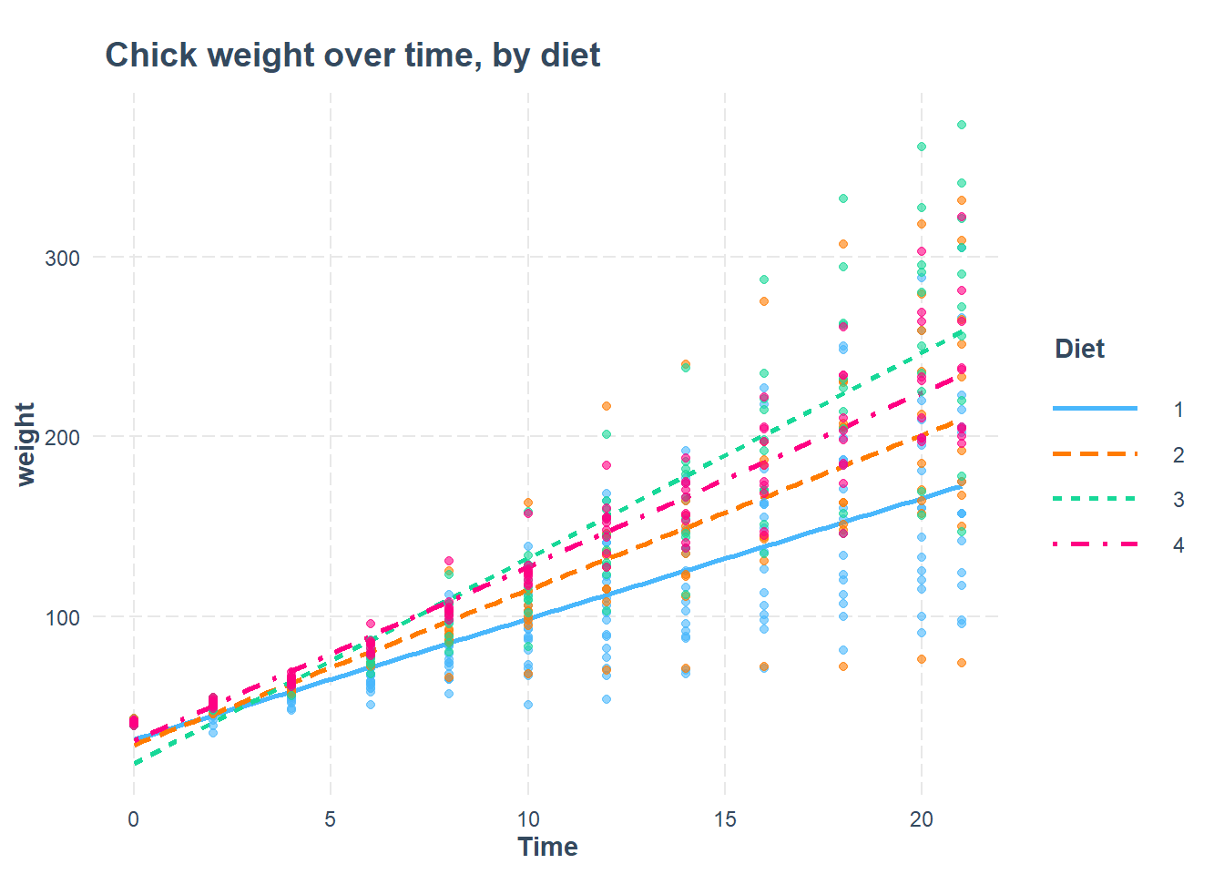

12.7 Assignment

In this assignment, you will answer a longitudinal research question using fixed effects and random effects models. You will explore the structure of the data, run visualizations, do an ICC calculation, create the regression models, and compare the regression models to each other.

Please download the data for this week’s assignment from D2L. The file is called CurranLong.sav.

Have a look at the following information about this dataset:²⁰⁷

The data are a sample of 405 children who were within the first two years of entry to elementary school. The data consist of four repeated measures of both the child’s antisocial behavior and the child’s reading recognition skills. In addition, on the first measurement occasion, measures were collected of emotional support and cognitive stimulation provided by the mother. The data were collected using face-to-face interviews of both the child and the mother at two-year intervals between 1986 and 1992.

Next, use this exact code to load the data:

if (!require(foreign)) install.packages('foreign')
library(foreign)

df <- read.spss("CurranLong.sav", to.data.frame = TRUE)

In this assignment, you will investigate the following research question: What is the change in reading ability of students over time?

Here is some information about the variables you should use:

• Dependent variable: read
• Key independent variable of interest: occasion

12.7.1 Data Structure

The first set of tasks is about exploring the structure of the data used in this assignment and relating it to previous data structures of multilevel data that we have encountered.

Task 1: Use the View() command to look at the dataset. What does each row of the data mean?

Task 2: List two variables in the data that vary from measurement to measurement of each subject. (In other words, list two variables that vary within subjects).

Task 3: List two variables in the data that do not vary from measurement to measurement of each subject. (In other words, list two variables that only vary between subjects).

Task 4: What is the Level 1 unit of observation in this data?

Task 5: What is the Level 2 unit of observation in this data?

Task 6: Write a standardized dataset description for the data you are using in this assignment.

Task 7: Using the appropriate descriptive tool, figure out how many rows in the data are measurements for occasion 0, 1, 2, and 3.

Task 8: Is our research question a within-subjects or between-subjects research question?

12.7.2 Visualization

Before you begin your analysis, it is important to visualize the data, like we did in the example earlier in this chapter.

Task 9: Create separate scatterplots for the observations in just the first 99 rows of the data.

Task 10: Which within-subject trends do you see in these plots?

Task 11: Which between-subject trends do you see in these plots?

Task 12: Using boxplots, examine the overall trend in read across occasion.

12.7.3 ICC

Now you will calculate the ICC for this data and outcome of interest in a number of ways.

Task 13: Make a null model for your research question. Call this mod0.

Task 14: Show how the ICC is calculated for this model (show the formula with the correct numbers plugged in).

Task 15: Calculate the ICC using R, to check your work above.

Task 16: Interpret the ICC for this model.

12.7.4 Fixed Effects Regression

Now you will run a fixed effects regression model to answer our research question.

Task 17: Run a fixed effects regression model to answer the research question, using plm(). Call this mod1. Interpret the results.

Task 18: Create an output table containing the intercepts from the fixed effects model and then inspect these intercepts. Include any of your observations.

Task 19: Add two more independent variables from the dataset to your fixed effects model. Interpret the results. Call this mod2. This may not always work, depending on which variables you choose. It is fine to skip this task if the model does not run correctly.

12.7.5 Random Effects Regression

In this part of the assignment, you will run both random intercepts and random slopes regression models to answer our research question.

Task 20: Run a random intercepts regression model to answer the research question. Call this mod3. Interpret the results.

Task 21: Show and inspect the coefficients of mod3. Include any of your observations.

Task 22: Run a random slopes regression model to answer the research question. Call this mod4. Interpret the results.

Task 23: Show and inspect the coefficients of mod4. Include any of your observations.

Task 24: Add two more independent variables from the dataset to mod4. Interpret the results. Call this mod5.

12.7.6 Confidence Intervals

Task 25: Report 95% confidence intervals of the coefficient estimates for the regression models that you ran. If you did not already include population interpretations in your earlier answers, please choose at least one regression model now and interpret its population-level results. If you want, you can do this all at once using stargazer, as demonstrated earlier.

12.7.7 Diagnostics

It is important to get in the habit of checking diagnostic tests after every single regression we run. Since this is your second time using both fixed effects and random effects, this time we will include some diagnostic tests.

Task 26: Check for multicollinearity in mod5

Task 27: Check for heteroscedasticity of the residuals of mod5, using visual inspection. The following code will produce a residuals versus fitted values plot for you: plot(mod5).

12.7.8 Additional items

You have now reached the end of this week’s assignment. The tasks below will guide you through submission of the assignment, remind you of any other items you need to complete this week, and allow us to gather questions and/or feedback from you.

Task 28: You are required to complete 15 quiz question flashcards in the Adaptive Learner App by the end of this week.

Task 29: Please write any questions you have for the course instructors (optional).

Task 30: Please write any feedback you have about the instructional materials (optional).

Task 31: Knit (export) your RMarkdown file into a format of your choosing.

Task 32: Please submit your assignment to the D2L assignment drop-box corresponding to this chapter and week of the course. And remember that if you have trouble getting your RMarkdown file to knit, you can submit your RMarkdown file itself. You can also submit an additional file(s) if needed.

---

203. Bates et al. Fitting Linear Mixed-Effects Models Using lme4. https://cran.r-project.org/web/packages/lme4/vignettes/lmer.pdf↩︎

204. Source: Section 1.2 “Example” in Bates et al. Fitting Linear Mixed-Effects Models Using lme4. https://cran.r-project.org/web/packages/lme4/vignettes/lmer.pdf↩︎

205. In the future, you might find yourself in a situation in which all of the repeated measures for one subject are in the same row of data. This is called wide format data. You need to reshape this data to long format data before you can analyze your data in the manner described in this chapter. There are multiple ways to do this in R.↩︎

206. Remember that R calls categorical variables “factor” variables. You can run the command class(sleepstudy$Subject) and R will tell you that the Subject variable is a factor.↩︎

207. Source: Multilevel Analysis. Utrecht University. https://multilevel-analysis.sites.uu.nl/datasets/↩︎